Preview Book "From 0day to CISM"

This section offers a look at Chapter 2 of From 0day to CISM – Certified Information Security Manager, a comprehensive study guide designed to prepare professionals for the CISM certification by ISACA. Bridging the gap between hands-on cybersecurity experience and executive-level information security knowledge, this book delivers a focused and structured approach to mastering essential CISM domains.

The preview below introduces key risk management concepts—such as risk appetite, tolerance, assessment, and treatment—highlighting their critical role in aligning security initiatives with business objectives.

1. Download the preview in a PDF format: Preview_Chapter_2_-_Information_Security_Risk_Management.pdf

2 INFORMATION SECURITY RISK MANAGEMENT

2.1          Introduction to Information Security Risk Management

Information security risk management is a core responsibility of security leaders, equipping them with processes to identify, assess, and mitigate risks that threaten an organization’s information assets. Effective risk management ensures that limited resources (time, budget, personnel) are prioritized toward the most significant security risks. In fact, maintaining an organization’s risk management program is one of the four primary domains of the Certified Information Security Manager (CISM) exam, reflecting its importance to the security manager’s role. This chapter provides a comprehensive overview of risk management concepts and practices, including risk assessment techniques, risk treatment options, security control categories, and frameworks (with a focus on NIST), as well as tools for risk visibility like risk registers. The goal is to build a solid understanding of how to manage cybersecurity risks in an enterprise environment, with special attention to exam-relevant formulas and concepts that CISM candidates should master.

Before diving into process and methodology, it is important to establish a clear vocabulary for discussing risk. In everyday conversation people often use terms like threat, vulnerability, and risk interchangeably, but in information security they have distinct meanings:

·         Threat: A threat is any external event or force that could potentially harm an information system. Threats can be natural (e.g. hurricanes, earthquakes, floods) or man-made (e.g. hackers, malware, terrorism). An easy way to think of a threat is as what we’re trying to protect against – it is a danger that exists independently of the organization’s control. For example, an earthquake or a hacker exists whether or not your organization is present; you generally cannot eliminate the existence of threats. A related term often used is threat vector, which describes the method or path a threat actor uses to reach a target (for instance, phishing emails, an exploit kit, or even physical break-in are all threat vectors).

·         Vulnerability: A vulnerability is a weakness or gap in our protections that could be exploited by a threat. In other words, vulnerabilities are internal factors – deficiencies in security controls, configurations, or processes – that leave an asset exposed to harm. Examples include an unpatched software flaw, an open network port, weak passwords, or an unlocked door. Unlike threats, organizations do have control over their vulnerabilities; a major part of security management is finding and fixing these weaknesses.

·         Risk: Risk arises only when a threat and a vulnerability are present simultaneously. A risk is the potential for loss or damage when a threat exploits a vulnerability. If either the threat or the vulnerability is absent, there is no risk (or effectively zero risk for that scenario). For example, if you have a server that is missing critical patches (vulnerability) and there are hackers actively seeking to exploit that software flaw (threat), then your organization faces a risk of compromise. Conversely, if your data center is inland and far from any coast, then even if the building construction is not hurricane-resistant (vulnerability), the risk of hurricane damage is negligible because the threat of a hurricane in that region is essentially non-existent. Likewise, you might have an external threat like a new computer virus in the wild, but if your systems are fully patched and have up-to-date antivirus (no vulnerability), that specific risk is mitigated. In short, risk is the possibility of harm materializing when a matching threat and vulnerability meet.

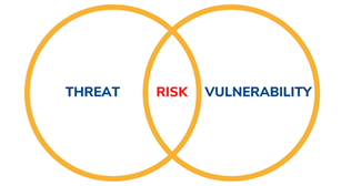
Figure: The image shows how threats, vulnerabilities, and risks are linked. A threat is a potential cause of harm, such as a cyberattack. A vulnerability is a weakness in a system that can be exploited by that threat. When a threat successfully exploits a vulnerability, it creates a risk — the possibility of loss or damage. Understanding this relationship is essential for assessing and managing cybersecurity risks effectively.

Once risks are identified, they are evaluated on two dimensions: likelihood and impact. The likelihood (or probability) of a risk event is the chance that the threat will exploit the vulnerability and materialize into an incident. For example, consider the risk of an earthquake affecting two different offices: one in California and one in Wisconsin. Historically, California experiences frequent earthquakes, whereas Wisconsin has had virtually none. Thus, the likelihood of earthquake damage is high in California and extremely low in Wisconsin. A risk manager in California must account for earthquakes as a realistic risk, whereas in Wisconsin that risk might be so unlikely that it can be deprioritized. The impact of a risk is the magnitude of damage or loss if the risk event occurs. For instance, an earthquake could cause catastrophic damage to a data center (high impact), while a minor rainstorm might cause negligible damage (low impact). Impact can be measured in various terms – commonly financial cost, but also reputational damage, regulatory penalties, safety consequences, etc., depending on the scenario.

Risk assessment is the process of analyzing identified risks by estimating their likelihood and impact, and then prioritizing them. The outcome of risk assessment is typically a ranked list of risks – so that management can focus on the most probable and harmful events first. There are two broad approaches to risk assessment: qualitative and quantitative. We will explore each in detail.

2.2          Risk Assessment Approaches

2.2.1    Qualitative Risk Assessment

Qualitative risk assessment uses subjective ratings to evaluate risk likelihood and impact, often expressed in relative terms such as “Low,” “Medium,” or “High.” Rather than assigning numeric values, qualitative methods rely on expert judgment, experience, and categorical scales to prioritize risks. This approach is common when exact data is scarce or when an organization wants a high-level overview of its risk landscape.

A popular tool in qualitative analysis is the risk matrix (also known as a heat map). This is a grid that plots likelihood on one axis and impact on the other, classifying risks into categories like low, moderate, or high based on where they fall in the grid. For example, an event that is assessed as having a High likelihood and High impact would be rated as a High Risk overall, demanding urgent attention. On the other hand, a risk with Medium likelihood but Low impact might be categorized as Low Risk overall, and thus not a top priority.

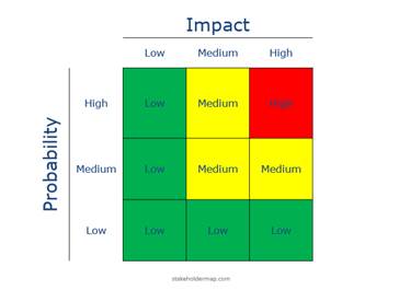
Figure: An example of a qualitative risk heat map. Likelihood is on the vertical axis (from Low at the bottom to High at the top), and Impact on the horizontal axis (from Low on the left to High on the right). Each cell’s color indicates the risk level – for instance, green for low risk, yellow for medium, and red for high. In this illustration, only combinations of high impact with medium or high likelihood yield High Risk (red). Notice that if either impact or likelihood is low (e.g. the bottom row, or the leftmost column), the overall risk is rated Low (green) despite the other factor.

Using such a matrix, an assessor can take each identified risk and assign it a qualitative likelihood rating and impact rating. These ratings are then combined (by rules defined in the matrix) to produce an overall risk rating. The matrix provides a visual cue to decision-makers: the clustering of risks in the red (high) zone versus yellow or green zones helps leadership immediately see which risks are most critical. Qualitative rankings are easy for stakeholders to understand and are very useful in facilitating discussions and initial prioritization.

However, qualitative assessments have limitations. They are inherently subjective – one expert’s "Medium" impact could be another’s "High." To improve consistency, organizations define risk rating criteria in their risk management policies. For example, impact criteria might be defined such that High impact means “financial loss over $1M or regulatory fines, or lives at stake,” Medium might mean “disruption of a major system or moderate financial loss,” and Low means “minor inconvenience or low cost.” Similarly, likelihood criteria might be tied to frequencies (e.g., High likelihood = expected to occur at least once a year, Medium = once every few years, Low = less than once in 10 years). By clearly defining these categories, qualitative assessments become more repeatable. Still, they remain coarse estimates.

2.2.2    Quantitative Risk Assessment

Quantitative risk assessment attempts to assign numeric values to both likelihood and impact, enabling the calculation of concrete financial risk figures. This approach relies on data: historical incident rates, statistical models, and asset valuations. The result is often expressed in monetary terms, which can be very powerful for cost-benefit analysis and communicating with executives in financial language.

The classic quantitative risk analysis methodology comes from the field of insurance and can be broken down into a few key metrics and formulas:

·         Asset Value (AV): The monetary value of the asset at risk. This could be the replacement cost of a piece of hardware, the assessed value of data or intellectual property, or any quantifiable value measure. For example, if we have a data center, we might determine that building a similar facility from scratch would cost $20 million; that figure would be our asset value for the data center.

·         Exposure Factor (EF): The proportion of the asset value that would be lost if a particular risk event occurs. EF is expressed as a percentage of damage. Different threats can have different exposure factors for the same asset. For instance, we might estimate that a major flood could destroy 50% of the data center’s equipment (EF = 0.5 or 50% damage), whereas a minor flood might only damage 10%. If a threat would likely destroy an asset completely, EF could be 100%. In our data center example, for a severe flood scenario we set EF = 50%.

·         Single Loss Expectancy (SLE): This is the expected monetary loss if the risk event occurs once. It is calculated as:

SLE = Asset Value × Exposure Factor

Using our numbers: AV = $20 million (data center), EF = 50% (flood damage). The SLE for a flood at the data center would be $20,000,000 × 0.5 = $10 million. In other words, a single flood incident is expected to cause $10M in damage. This represents the impact in financial terms for one occurrence of that risk.

·         Annualized Rate of Occurrence (ARO): This is the estimated frequency with which we expect the risk event to occur, expressed on a yearly basis. An ARO of 1.0 means once per year on average; 0.5 would mean once every two years; 0.01 means once every 100 years, and so on. Determining ARO often involves historical data or industry statistics. In our example, we might consult meteorological data (such as FEMA flood maps) to find the probability of a severe flood in the area. Suppose it’s a 1% chance per year (a "100-year floodplain"). That corresponds to an ARO of 0.01 for the flood risk.

·         Annualized Loss Expectancy (ALE): This is the key result of quantitative risk analysis – the expected monetary loss per year from a given risk. ALE is calculated by multiplying SLE by ARO:

ALE = SLE × ARO

Continuing our example: SLE = $10,000,000, ARO = 0.01. Thus ALE = $10,000,000 × 0.01 = $100,000 per year. This means, on average, the organization can expect $100k in losses each year due to data center flooding. Of course, in reality the flood will not happen every year – what this says is that over a long period (say 100 years) you’d expect one $10M incident, which averages out to $100k per year. ALE provides a way to annualize risk for budgeting and decision-making purposes.

To summarize the formulas:

Beyond monetary risk calculations, quantitative analysis often extends to other numeric metrics that inform risk and continuity planning. In IT operations and disaster recovery contexts, you should understand the following measures of reliability and resilience:

·         Mean Time to Failure (MTTF): The average time expected until a non-repairable asset fails. For devices or components that are not repaired upon failure (they are simply replaced), MTTF indicates reliability. For example, if a particular model of hard drive has an MTTF of 100,000 hours, that is the average lifespan – half the drives would fail before that time and half after (by definition of an average). MTTF is used for planning maintenance and replacements.

·         Mean Time Between Failures (MTBF): For repairable systems, which can be fixed and returned to service after a failure, MTBF measures the average time between one failure and the next. It is conceptually similar to MTTF, but applies when the item is restored rather than replaced. For instance, if a server tends to crash and be repaired, an MTBF of 200 days means on average it goes 200 days between incidents. Higher MTBF indicates more reliable systems.

·         Mean Time to Repair (MTTR): This is the average time it takes to repair a system or component and restore it to operation after a failure. If a system has an MTTR of 4 hours, that means typically it takes 4 hours to get it back online each time it fails. MTTR is crucial for understanding downtime duration and for continuity plans (e.g., how long will a service be unavailable when an incident occurs?).

Using MTBF and MTTR together helps assess the expected availability of a system. For example, if a system fails on average every 200 days (MTBF) and takes 4 hours to recover (MTTR), over a year you can estimate the total downtime and plan accordingly. These metrics also tie into calculating service availability percentages and making decisions about redundancy and maintenance.

In summary, quantitative risk assessment provides hard numbers that can guide cost-benefit decisions. If the ALE of a risk is $100k, and a proposed control (like building a flood wall) costs $1M, a manager can compare those figures to decide if the control is economically justified. Often, organizations will use a combination of qualitative and quantitative methods – qualitative for broad initial assessment and when quantitative data is lacking, and quantitative for high-value assets or when making the business case for specific investments.

2.3          Information Classification and Asset Criticality

An important facet of risk management is understanding what you are protecting and how important it is. This is where information classification comes into play. Organizations use classification schemes to label data and systems according to their sensitivity and criticality, which in turn drives the security requirements for handling and protecting that information. In essence, not all data is equal – losing some pieces of information could be a minor inconvenience, while losing others could be a catastrophic event. Classification helps set the level of protection proportionate to the value or impact of loss of the asset.

Classification policies define categories or levels of sensitivity. Each level in the scheme has associated handling standards (who can access it, how it must be stored, whether it needs encryption, etc.). While each organization’s scheme can differ, they typically map to the concept of high, medium, or low sensitivity information. For example, many government agencies use the classic hierarchy: Unclassified, Confidential, Secret, Top Secret, where Top Secret information could cause grave damage if disclosed, and Unclassified is essentially public information. Private sector businesses often use analogous categories with different labels, such as Public, Internal, Sensitive, Highly Sensitive, etc., to classify their proprietary and customer data.

For instance, consider a possible mapping between government and corporate classification levels:

The exact names and number of levels can vary. The key point is that classified information must be handled according to its level. For example, a company might mandate that any data labeled Highly Sensitive must be encrypted in transit and at rest, stored only on approved secure servers, and accessible only by a need-to-know list of employees. Less sensitive data might not require encryption or might be allowed on public cloud storage, etc. The classification triggers appropriate controls. Additionally, organizations will often label data (both digital and physical) to indicate its classification – e.g., emails might have a header like “Internal – Company Confidential” or documents stamped “Proprietary” – so that users are aware of handling requirements.

Certain types of data carry legal or regulatory implications, and these often warrant a high classification. For example, personally identifiable information (PII) about customers, financial records (like credit card numbers), and health records (subject to laws like HIPAA) are often treated as highly sensitive regardless of internal value, because their compromise triggers regulatory penalties and reputational damage. Thus, an organization’s classification policy should consider not just the impact to the organization, but also impact to individuals whose data is compromised. Protection of customer data and privacy information is a critical part of risk management today.

Implementing a classification scheme can be challenging. It typically starts with a thorough inventory of information assets – identifying what data exists and where – which can be labor intensive. But the payoff is a structured understanding of where the crown jewels are, so to speak, enabling focused security controls on those areas. Classification is foundational: it feeds into risk assessment (by identifying which assets are high-value) and into control selection (by specifying baseline controls for each level). In fact, in formal risk management frameworks like NIST, categorizing information and systems is Step 1 of the process. We will see this again when discussing the NIST Risk Management Framework.

2.4          Risk Treatment Options

After completing a risk assessment, you will have a list of identified risks with their assessed likelihoods and impacts. The next challenge is deciding how to address each risk. This process is known as risk treatment or risk response. For any given risk, there are four general strategies an organization can choose from:

1.       Risk Avoidance: Avoidance means eliminating the risk entirely by ceasing the activities that create the risk. In practice, this often involves changing business plans or processes so that the risky situation is no longer encountered. For example, if an organization’s data center is in a flood zone and faces high flood risk, an avoidance strategy would be relocating the data center to a place with no flood hazard. By doing so, the risk of flood damage is removed (avoided). Avoidance is a very effective strategy in terms of risk elimination, but it can come at the cost of giving up certain opportunities or benefits (in this case, perhaps the convenience or low cost of the original location). Organizations should consider avoidance when a risk is too dangerous or costly to mitigate by other means and if the activity causing the risk is not mission-critical.

2.       Risk Transference (Risk Sharing): Transference means shifting the impact of the risk to a third party. The most common form is purchasing insurance. When you buy insurance (cyber insurance, property insurance, etc.), you are transferring the financial impact of certain losses to the insurer – if the bad event occurs, the insurance company pays the bill (up to a limit), not you. Another example is outsourcing: if a company outsources a service, some risks associated with that service (and its security) might be transferred contractually to the vendor. However, it is important to note that not all aspects of risk can be transferred. Using the data center flood example, you could purchase flood insurance to cover the financial losses of equipment damage, but you cannot transfer the reputational damage or operational downtime easily – those residual impacts still affect your organization. Transference is a useful strategy for risks that can be clearly defined and priced (hence insurable), or where specialized third parties can manage the risk more effectively.

3.       Risk Mitigation: Mitigation (or risk reduction) involves taking active steps to reduce the likelihood and/or impact of the risk. This is the heart of most cybersecurity efforts – implementing controls and countermeasures to treat the risk. For example, to mitigate the flood risk to the data center, the company might invest in flood control measures: installing water diversion systems, pumps, raised barriers, etc., to reduce the chance that flood waters reach critical equipment. In cybersecurity, nearly all security controls (firewalls, antivirus, encryption, backups, etc.) are risk mitigations – they don’t remove the threat and might not fix every vulnerability, but they lower the risk to an acceptable level by making incidents less likely or less damaging. Mitigation is the most commonly chosen approach for a majority of identified risks because it allows business to continue while improving safety.

4.       Risk Acceptance: Acceptance means acknowledging the risk and choosing to take no special action to address it, apart from monitoring. This might sound counterintuitive – why would you ever accept a risk? In reality, organizations face hundreds of risks, and it is not feasible to avoid, transfer, or mitigate all of them. Some risks will be deemed low enough (in likelihood or impact) that the cost or effort of treating them outweighs the potential damage. For instance, after considering various options, the company might decide that the flood risk (especially if low probability) is something they will simply live with – perhaps all other options (moving the data center, buying insurance, installing flood controls) are too expensive or impractical, so they accept the risk and will deal with a flood if and when it happens. Risk acceptance should be a conscious, documented decision, ideally made by senior management, not an oversight. It’s essentially saying “we can tolerate this risk at its current level.” It’s important that accepted risks are monitored in case their status changes (for example, if what was once a low risk becomes more likely or more impactful, it may no longer be acceptable).

Every risk must be dealt with using one or a combination of these strategies. In some cases, multiple strategies apply – for example, an organization might mitigate most of a risk and then insure (transfer) the residual impact. Or it might avoid part of a risk and accept the rest. The combination of all risks an organization faces is often called its risk profile. Management’s job is to choose an appropriate mix of responses so that the overall risk profile is in line with the organization’s objectives and capabilities.

Two important terms related to choosing risk responses are inherent risk and residual risk. Inherent risk is the level of risk that exists before any controls or treatments are applied – essentially the raw, unmitigated risk. Residual risk is the level of risk that remains after controls are implemented. Ideally, your mitigation efforts significantly reduce a high inherent risk down to a lower residual risk. For example, inherently a data center in a floodplain has a high risk of flood damage. If you install flood gates and pumps (mitigations), the residual risk might drop to moderate. There will almost always be some residual risk, because it's rare to eliminate a risk entirely short of avoiding it altogether.

One more concept: introducing new controls can sometimes create new risks of their own – this is known as control risk. For instance, adding a firewall mitigates many network threats, but it introduces the risk that the firewall could fail or even malfunction and block legitimate traffic. Similarly, complexity from many controls might introduce system bugs or administrative mistakes. These control-induced risks must be considered as part of the analysis. The goal of risk management is to ensure that residual risk + control risk remains within the organization’s tolerance.

Speaking of tolerance, organizations determine how much risk they are willing to accept – this is referred to as risk appetite. Senior leadership and the board will set the overall risk appetite: for example, a company might decide it is comfortable with low to moderate risks in most areas but has zero tolerance for risks that could endanger human life or violate laws. Risk appetite guides decisions on which risks to mitigate and how much to spend on controls. If the residual risk of some activity exceeds the risk appetite (meaning it's too high for comfort even after mitigations), then additional controls or different strategies (like avoidance) should be pursued until risk is reduced to acceptable levels.

2.5          Security Control Selection and Implementation

Once risk treatment decisions are made (especially decisions to mitigate), the next step is to select and implement appropriate security controls. Security controls (also called countermeasures or safeguards) are the measures taken to modify risk – typically by protecting assets or reducing the likelihood/impact of incidents. As a security manager, a large portion of your job involves designing, implementing, and overseeing these controls.

It’s useful to think of security controls in everyday terms first. Consider how you secure your home: you likely have locks on doors and windows to prevent intrusions, maybe an alarm system to detect break-ins, security cameras to record events, perhaps automatic lights to deter criminals by simulating occupancy, and even policies like asking a neighbor to check your mail when you’re on vacation. Each of these is a control addressing a certain risk (burglary in this case) in a certain way. Some controls overlap in purpose – for example, both the alarm and the cameras are aimed at detecting intruders. You might intentionally have multiple controls for the same risk as a safety net in case one fails – if the alarm doesn’t go off, the cameras might still catch the thief. In security parlance, this is known as defense in depth: implementing multiple layers of controls so that if one layer fails, others still protect the asset.

When managing enterprise security, we categorize controls in a couple of different and complementary ways. Understanding these categories is important both for design (to ensure you have a balanced security program) and for exam purposes (CISM may ask about types of controls and their characteristics).

2.5.1    Control Categories by Purpose (Function)

This classification is based on what the control is intended to do in the risk management lifecycle. Common functional categories include:

·         Preventive Controls: These are designed to stop an incident from occurring in the first place. They act before a threat can actually impact an asset. Examples: a firewall blocking unauthorized network traffic is a preventive technical control that stops attacks at the network border; door locks and badges prevent unauthorized physical entry (a preventive physical control); security policies and training can be preventive administrative controls by discouraging unsafe behaviors. Essentially, anything that reduces the likelihood of a security breach upfront is preventive.

·         Detective Controls: These aim to identify or discover incidents (or signs of an imminent incident) so that you can respond. They come into play during or after an incident, when prevention has not been fully successful. Examples: an intrusion detection system (IDS) that generates an alert upon suspicious network activity is detective; security cameras or motion sensors detect physical intrusions; log monitoring systems and audits detect irregularities or malicious activity in systems. Detective controls do not stop an incident by themselves, but they are crucial for awareness – you cannot respond to what you don’t know about.

·         Corrective Controls: These are designed to limit damage and restore systems after an incident has occurred. They minimize impact (assuming preventive controls were bypassed and an incident happened). Examples: data backups are a corrective control – if ransomware encrypts your files, you restore from backup to recover; a patch management process is corrective when it removes vulnerabilities (fixing the condition that allowed an incident); incident response procedures themselves are corrective actions to contain and eradicate a threat. A fire extinguisher is a non-digital example of a corrective control (putting out a fire to minimize damage).

·         Deterrent Controls: (Sometimes listed separately) These are controls that discourage attackers by making the effort riskier or less appealing. They overlap with preventive in effect, but their main function is psychological. Examples: Security cameras and warning signs can act as deterrents (even if they also have a detective function); a prominently displayed legal banner on a system warning of prosecution might deter casual malicious behavior. Deterrents often complement other controls.

·         Compensating Controls: (Special category) These are alternative controls that provide equivalent protection when the primary recommended control is not feasible. For instance, if a system cannot support encryption (primary control), you might compensate with extra network segregation and monitoring to achieve an equivalent risk reduction. Compensating controls don’t neatly fit in prevent/detect/correct – they are basically substitute controls.

Most discussions focus on Preventive, Detective, and Corrective as the main three functions (with deterrent sometimes considered a subset of preventive, and compensating being a design choice when needed). A strong security program uses a blend of all three: you want to prevent what you can, detect the things you couldn’t prevent, and correct the issues that are detected – all in layers.

2.5.2    Control Categories by Nature (Implementation)

This classification is based on how the control is implemented or what form it takes:

·         Technical Controls (Logical Controls): These are controls implemented through technology and systems (hardware, software, or firmware). They operate within IT systems. Examples: encryption of data, access control mechanisms in software, firewalls, antivirus software, intrusion prevention systems, multi-factor authentication – all are technical controls. They enforce security through technical means with minimal human intervention in operation.

·         Operational Controls (Procedural Controls): These are processes and procedures carried out by people (often IT or security staff, but sometimes end-users or managers) to maintain security. They often support technical controls. Examples: conducting regular log reviews, performing background checks on new hires, monitoring CCTV feeds, incident response drills, user security awareness training, change management processes. These activities require human execution and oversight. Sometimes physical security measures (guards, facility procedures) are lumped into operational controls as well, since they are about day-to-day operations.

·         Managerial Controls (Administrative Controls): These are high-level governance and policy oriented controls, usually documented in plans, policies, and procedures that guide the organizational approach to security. They set the framework and oversight for other controls. Examples: risk assessment processes (yes, performing a risk assessment is itself a security control of managerial type), security policy documentation, vendor assessment procedures, security architecture reviews, change control boards, audit committees, etc. Managerial controls ensure that security is designed and managed properly throughout the organization.

·         Physical Controls: (Often considered a subset of technical or operational, but worth noting separately) These are controls that physically restrict or protect access to information or resources. Examples: locks, fences, security guards, badge access systems, video surveillance, fire suppression systems, climate controls to protect hardware, etc. Physical controls usually work in tandem with technical measures to secure the actual facilities and hardware.

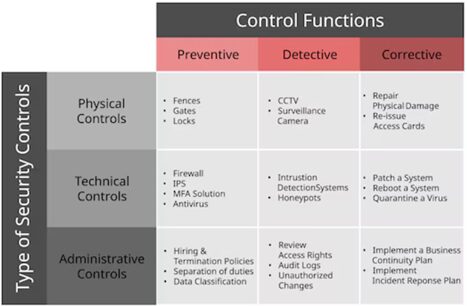
Figure: The figure categorizes cybersecurity controls into physical, technical, and administrative types, each serving different functions: preventive, detective, and corrective. Preventive controls aim to stop incidents before they occur, such as gates and firewalls. Detective controls are designed to identify and monitor incidents, like CCTV systems or audit logs. Corrective controls focus on responding to and recovering from incidents, for example by patching systems or implementing an incident response plan. This structured approach helps organizations address threats across multiple layers of defense.

In the literature, you may see the triad administrative, technical, physical as categories – administrative corresponds to our managerial/operational policies; technical to logical controls; physical remains physical. The NIST approach mentioned in the content above groups into technical, operational, and management, implicitly covering physical under operational.

It’s important to have a mix of these implementation categories. For example, you might address the risk of unauthorized data access with technical controls (access control lists, encryption), operational controls (regular permission reviews by admins, training users on data handling), physical controls (locked server room), and managerial controls (an information security policy that defines access management procedures). Together, they form layers of defense.

When selecting controls, you often start with baseline controls (common safeguards applicable to most systems) and then tailor them to specific risks identified. Industry standards like ISO 27001 or NIST SP 800-53 provide catalogs of controls to consider. The selection must be appropriate to the risk’s magnitude (don’t use a sledgehammer for a fly, but also don’t bring a knife to a gunfight, as the sayings go). Cost-benefit analysis is part of this – you aim for controls where the benefit (risk reduction) justifies the cost, and that collectively bring risk down to acceptable levels.

Once implemented, controls need to be assessed for proper function. Even the best control on paper can fail if misconfigured. Two terms often come up regarding control efficacy: false positives and false negatives. A false positive occurs when a control triggers an alert or action when it shouldn’t – a benign activity is mistaken as malicious. For instance, an intrusion detection system that raises an alarm for normal network traffic is generating a false positive. False positives can lead to wasted effort and “alarm fatigue,” where admins might start ignoring alerts due to frequent bogus alarms. A false negative is the opposite: the control fails to trigger when it should, missing a real attack or incident. Using the IDS example, if a real intrusion happens but the IDS does not detect it, that is a false negative – far more dangerous because it gives a false sense of security. When tuning controls (like IDS rules, spam filters, etc.), there’s often a trade-off between false positives and false negatives; careful calibration is needed to minimize both.

In practice, after controls are in place, organizations conduct control assessments (which we’ll cover next) to ensure that controls are implemented correctly, operating as intended, and fulfilling their purpose. This is a continuous effort – security controls require monitoring and maintenance. For example, a firewall rule base might need periodic review, or user access permissions need to be re-certified regularly (an operational control to ensure the technical access control is still aligned with who should have access).

2.6          Ongoing Risk Management and Continuous Monitoring

. . .

<end of preview>